Usage
Simple example
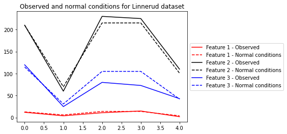
In the following, we use AAKR on Linnerud dataset, to find out values we expect to see in normal conditions for part of the dataset.
First, we import the necessary libraries.
from aakr import AAKR
from sklearn.datasets import load_linnerud
Second, we load the dataset and split it into two parts:
X_ncwith examples of normal conditionsX_obswith observed values, for which we want to find values we would’ve expected to see in normal conditions
# Load dataset (20 samples, 3 features)
X = load_linnerud().data

# Use first 15 as examples of normal conditions
X_nc = X[:15]

# New observations to get normal condition for
X_obs = X[15:]
Third, we create the AAKR model and fit the normal condition examples.
# Create AAKR and fit first 15 observations
aakr = AAKR()
aakr.fit(X_nc)
Fourth, we use transform to obtain the normal conditions.
# Normal conditions for the last 5 observations
X_obs_nc = aakr.transform(X_obs)
Finally, we plot the results.
# Plot results
import matplotlib.pyplot as plt

colors = 'rkb'
for i in range(X.shape[1]):
    plt.plot(X_obs[:, i], color=colors[i], linestyle='-',
            label=f'Feature {i + 1} - Observed')
    plt.plot(X_obs_nc[:, i], color=colors[i], linestyle='--',
            label=f'Feature {i + 1} - Normal conditions')

plt.title('Observed and normal conditions for Linnerud dataset')
plt.legend(loc='center left', bbox_to_anchor=(1, 0.5))
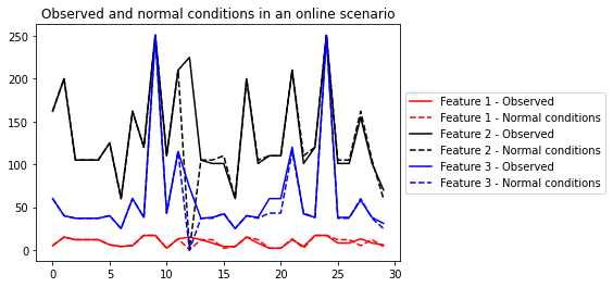
Online example
AAKR is well suited for scenarios where fit and predict needs to be performed as new values come in, e.g. from sensors. The following is an example of this kind of a scenario.
First, we create a data generator that simulates a sensor.
import numpy as np

from aakr import AAKR
from sklearn.datasets import load_linnerud

np.random.seed(2020)

def data_generator(n_iters=50):
    """Generates rows randomly from Linnerud dataset."""
    X = load_linnerud().data

    for i in range(n_iters):
        yield X[[np.random.choice(X.shape[0])]]
Second, we create a new instance of the model.
# Initiate model
aakr = AAKR()
Third, we iterate n_iters times over sensor values, where first n_train observations are used for fitting AAKR model one-by-one by utilizing the partial_fit -method. The results are saved into lists.
# Simulate data flow
n_train = 12  # Use first `n_train` observations for fitting
n_iters = 30  # Number of iterations from data generator

X = []
X_obs_nc = []
for i, X_obs in enumerate(data_generator(n_iters)):

    # Fit latest observation
    if i < n_train:
        aakr.partial_fit(X_obs)

    # Based on the history, what should we see in normal conditions
    X_obs_nc_latest = aakr.transform(X_obs)

    # Save original observation and normal condition values
    X.append(X_obs[0])
    X_obs_nc.append(X_nc[0])
Finally, we plot the results.
# Plot results
import matplotlib.pyplot as plt

X = np.array(X)
X_obs_nc = np.array(X_obs_nc)

colors = 'rkb'
for i in range(X.shape[1]):
    plt.plot(X[:, i], color=colors[i], linestyle=':',
            label=f'Feature {i + 1} - Observed')
    plt.plot(X_obs_nc[:, i], color=colors[i], linestyle='-',
            label=f'Feature {i + 1} - Normal conditions')

plt.title('Observed and normal conditions in an online scenario')
plt.legend(loc='center left', bbox_to_anchor=(1, 0.5))