aakr (Auto Associative Kernel Regression)

aakr is a Python implementation of the Auto-Associative Kernel Regression (AAKR). The algorithm is suitable for signal reconstruction, which can further be used for condition monitoring, anomaly detection etc.

Documentation is available at https://aakr.readthedocs.io.

Installation

pip install aakr

Quickstart

Given historical normal condition X_nc examples and new observations X_obs of size n_samples x n_features, what values we expect to see in normal conditions for the new observations?

from aakr import AAKR

# Create AAKR model
aakr = AAKR()

# Fit the model with normal condition examples
aakr.fit(X_nc)

# Ask for values expected to be seen in normal conditions
X_obs_nc = aakr.transform(X_obs)

References

• Assessment of Statistical and Classification Models For Monitoring EDF’s Assets

• A modified Auto Associative Kernel Regression method for robust signal reconstruction in nuclear power plant components

---

Jesse Myrberg (jesse.myrberg@gmail.com)

aakr (Auto Associative Kernel Regression)

aakr is a Python implementation of the Auto-Associative Kernel Regression (AAKR). The algorithm is suitable for signal reconstruction, which can further be used for condition monitoring, anomaly detection etc.

Documentation is available at https://aakr.readthedocs.io.

Installation

pip install aakr

Quickstart

Given historical normal condition X_nc examples and new observations X_obs of size n_samples x n_features, what values we expect to see in normal conditions for the new observations?

from aakr import AAKR

# Create AAKR model
aakr = AAKR()

# Fit the model with normal condition examples
aakr.fit(X_nc)

# Ask for values expected to be seen in normal conditions
X_obs_nc = aakr.transform(X_obs)

References

• Assessment of Statistical and Classification Models For Monitoring EDF’s Assets

• A modified Auto Associative Kernel Regression method for robust signal reconstruction in nuclear power plant components

---

Jesse Myrberg (jesse.myrberg@gmail.com)

Usage

Simple example

In the following, we use AAKR on Linnerud dataset, to find out values we expect to see in normal conditions for part of the dataset.

First, we import the necessary libraries.

from aakr import AAKR
from sklearn.datasets import load_linnerud

Second, we load the dataset and split it into two parts:

1. X_nc with examples of normal conditions

2. X_obs with observed values, for which we want to find values we would’ve expected to see in normal conditions

# Load dataset (20 samples, 3 features)
X = load_linnerud().data

# Use first 15 as examples of normal conditions
X_nc = X[:15]

# New observations to get normal condition for
X_obs = X[15:]

Third, we create the AAKR model and fit the normal condition examples.

# Create AAKR and fit first 15 observations
aakr = AAKR()
aakr.fit(X_nc)

Fourth, we use transform to obtain the normal conditions.

# Normal conditions for the last 5 observations
X_obs_nc = aakr.transform(X_obs)

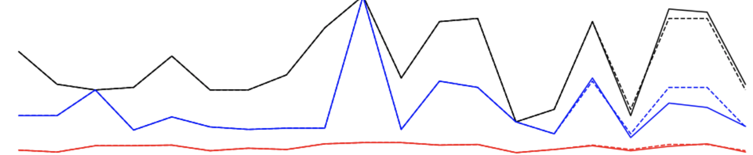
Finally, we plot the results.

# Plot results
import matplotlib.pyplot as plt

colors = 'rkb'
for i in range(X.shape[1]):
    plt.plot(X_obs[:, i], color=colors[i], linestyle='-',
            label=f'Feature {i + 1} - Observed')
    plt.plot(X_obs_nc[:, i], color=colors[i], linestyle='--',
            label=f'Feature {i + 1} - Normal conditions')

plt.title('Observed and normal conditions for Linnerud dataset')
plt.legend(loc='center left', bbox_to_anchor=(1, 0.5))

Online example

AAKR is well suited for scenarios where fit and predict needs to be performed as new values come in, e.g. from sensors. The following is an example of this kind of a scenario.

First, we create a data generator that simulates a sensor.

import numpy as np

from aakr import AAKR
from sklearn.datasets import load_linnerud

np.random.seed(2020)

def data_generator(n_iters=50):
    """Generates rows randomly from Linnerud dataset."""
    X = load_linnerud().data

    for i in range(n_iters):
        yield X[[np.random.choice(X.shape[0])]]

Second, we create a new instance of the model.

# Initiate model
aakr = AAKR()

Third, we iterate n_iters times over sensor values, where first n_train observations are used for fitting AAKR model one-by-one by utilizing the partial_fit -method. The results are saved into lists.

# Simulate data flow
n_train = 12  # Use first `n_train` observations for fitting
n_iters = 30  # Number of iterations from data generator

X = []
X_obs_nc = []
for i, X_obs in enumerate(data_generator(n_iters)):

    # Fit latest observation
    if i < n_train:
        aakr.partial_fit(X_obs)

    # Based on the history, what should we see in normal conditions
    X_obs_nc_latest = aakr.transform(X_obs)

    # Save original observation and normal condition values
    X.append(X_obs[0])
    X_obs_nc.append(X_nc[0])

Finally, we plot the results.

# Plot results
import matplotlib.pyplot as plt

X = np.array(X)
X_obs_nc = np.array(X_obs_nc)

colors = 'rkb'
for i in range(X.shape[1]):
    plt.plot(X[:, i], color=colors[i], linestyle=':',
            label=f'Feature {i + 1} - Observed')
    plt.plot(X_obs_nc[:, i], color=colors[i], linestyle='-',
            label=f'Feature {i + 1} - Normal conditions')

plt.title('Observed and normal conditions in an online scenario')
plt.legend(loc='center left', bbox_to_anchor=(1, 0.5))

aakr package

Module contents

class aakr.AAKR(metric='euclidean', bw=1.0, modified=False, penalty=None, n_jobs=- 1)

Bases: sklearn.base.TransformerMixin, sklearn.base.BaseEstimator

Auto Associative Kernel Regression.

Parameters

• metric (str, default='euclidean') – Metric for calculating kernel distances, see available metrics from sklearn.metrics.pairwise_distances.

• bw (float, default=1.0) – Gaussian Radial Basis Function (RBF) bandwith parameter.

• modified (bool, default=False) – Whether to use the modified version of AAKR (see reference [2]). The modified version reduces the contribution provided by those signals which are expected to be subject to the abnormal conditions.

• penalty (array-like or list of shape (n_features, 1) or None, default=None) – Penalty vector for the modified AAKR - only used when parameter modified=True. If modified AAKR used and penalty=None, penalty vector is automatically determined.

• n_jobs (int, default=-1) – The number of jobs to run in parallel.

X_

Historical normal condition examples given as an array.

Type

ndarray of shape (n_samples, n_features)

References

1

Chevalier R., Provost D., and Seraoui R., 2009, “Assessment of Statistical and Classification Models For Monitoring EDF’s Assets”, Sixth American Nuclear Society International Topical Meeting on Nuclear Plant Instrumentation.

2

Baraldi P., Di Maio F., Turati P., Zio E., 2014, “A modified Auto Associative Kernel Regression method for robust signal reconstruction in nuclear power plant components”, European Safety and Reliability Conference ESREL.

Methods

fit(X[, y])	Fit normal condition examples.
fit_transform(X[, y])	Fit to data, then transform it.
get_params([deep])	Get parameters for this estimator.
partial_fit(X[, y])	Fit more normal condition examples.
set_params(**params)	Set the parameters of this estimator.
transform(X)	Transform given array into expected values in normal conditions.

fit(X, y=None)

Fit normal condition examples.

Parameters

• X (array-like of shape (n_samples, n_features)) – Training examples from normal conditions.

• y (None) – Not required, exists only for compability purposes.

Returns

self – Returns self.

Return type

object

fit_transform(X, y=None, **fit_params)

Fit to data, then transform it.

Fits transformer to X and y with optional parameters fit_params and returns a transformed version of X.

Parameters

• X (array-like of shape (n_samples, n_features)) – Input samples.

• y (array-like of shape (n_samples,) or (n_samples, n_outputs), default=None) – Target values (None for unsupervised transformations).

• **fit_params (dict) – Additional fit parameters.

Returns

X_new – Transformed array.

Return type

ndarray array of shape (n_samples, n_features_new)

get_params(deep=True)

Get parameters for this estimator.

Parameters

deep (bool, default=True) – If True, will return the parameters for this estimator and contained subobjects that are estimators.

Returns

params – Parameter names mapped to their values.

Return type

dict

partial_fit(X, y=None)

Fit more normal condition examples.

Parameters

• X (array-like of shape (n_samples, n_features)) – Training examples from normal conditions.

• y (None) – Not required, exists only for compability purposes.

Returns

self – Returns self.

Return type

object

set_params(**params)

Set the parameters of this estimator.

The method works on simple estimators as well as on nested objects (such as Pipeline). The latter have parameters of the form <component>__<parameter> so that it’s possible to update each component of a nested object.

Parameters

**params (dict) – Estimator parameters.

Returns

self – Estimator instance.

Return type

estimator instance

transform(X)

Transform given array into expected values in normal conditions.

Parameters

X (array-like of shape (n_samples, n_features)) – The input samples.

Returns

X_nc – Expected values in normal conditions for each sample and feature.

Return type

ndarray of shape (n_samples, n_features)